Superposition as Lossy Compression – Measure with Sparse Autoencoders and Connect to Adversarial Vulnerability
An information-theoretic framework quantifying superposition as lossy compression in neural networks. By measuring effective degrees of freedom through sparse autoencoders, we reveal that adversarial training's effect on feature organization depends on task complexity relative to network capacity.
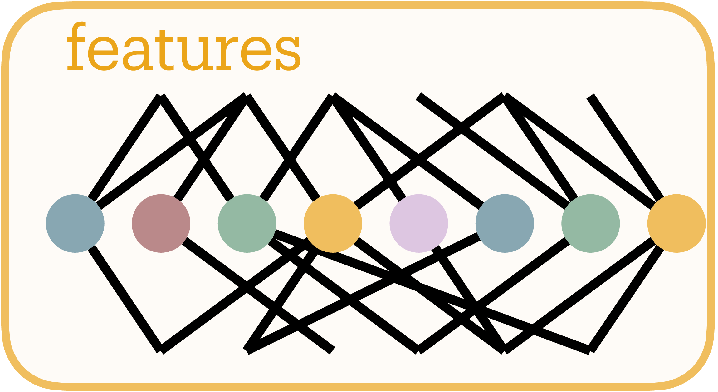
Neural networks achieve remarkable performance through superposition: encoding multiple features as overlapping directions in activation space rather than dedicating individual neurons to each feature. This phenomenon challenges interpretability; when neurons respond to multiple unrelated concepts, understanding network behavior becomes difficult. Yet despite its importance, we lack principled methods to measure superposition. We present an information-theoretic framework measuring a neural representation’s effective degrees of freedom. We apply Shannon entropy to sparse autoencoder activations to compute the number of effective features as the minimum number of neurons needed for interference-free encoding. Equivalently, this measures how many “virtual neurons” the network simulates through superposition. When networks encode more effective features than they have actual neurons, they must accept interference as the price of compression. Our metric strongly correlates with ground truth in toy models, detects minimal superposition in algorithmic tasks (effective features approximately equal neurons), and reveals systematic reduction under dropout. Layer-wise patterns of effective features mirror studies of intrinsic dimensionality on Pythia-70M. The metric also captures developmental dynamics, detecting sharp feature consolidation during the grokking phase transition. Surprisingly, adversarial training can increase effective features while improving robustness, contradicting the hypothesis that superposition causes vulnerability. Instead, the effect of adversarial training on superposition depends on task complexity and network capacity: simple tasks with ample capacity allow feature expansion (abundance regime), while complex tasks or limited capacity force feature reduction (scarcity regime). By defining superposition as lossy compression, this work enables principled, practical measurement of how neural networks organize information under computational constraints, particularly connecting superposition to adversarial robustness.
Introduction
Interpretability and adversarial robustness could be two sides of the same coin
The superposition hypothesis offers a potential mechanism. Elhage et al.
Testing this prediction requires measuring superposition in real networks. While Elhage et al.
We solve this through information theory applied to sparse autoencoders (SAEs). SAEs extract interpretable features from neural activations
The exponential of the Shannon entropy quantifies how many interference-free channels would transmit this feature distribution, the network’s effective degrees of freedom. We call this count effective features $F$ (Figure 2b): the minimum neurons needed to encode the observed features without interference. We interpret this as $F$ “virtual neurons”: the network simulates this many independent channels through its $N$ physical neurons (Figure 2b). The feature distribution compresses losslessly down to exactly $F$ neurons; compress further and interference becomes unavoidable.
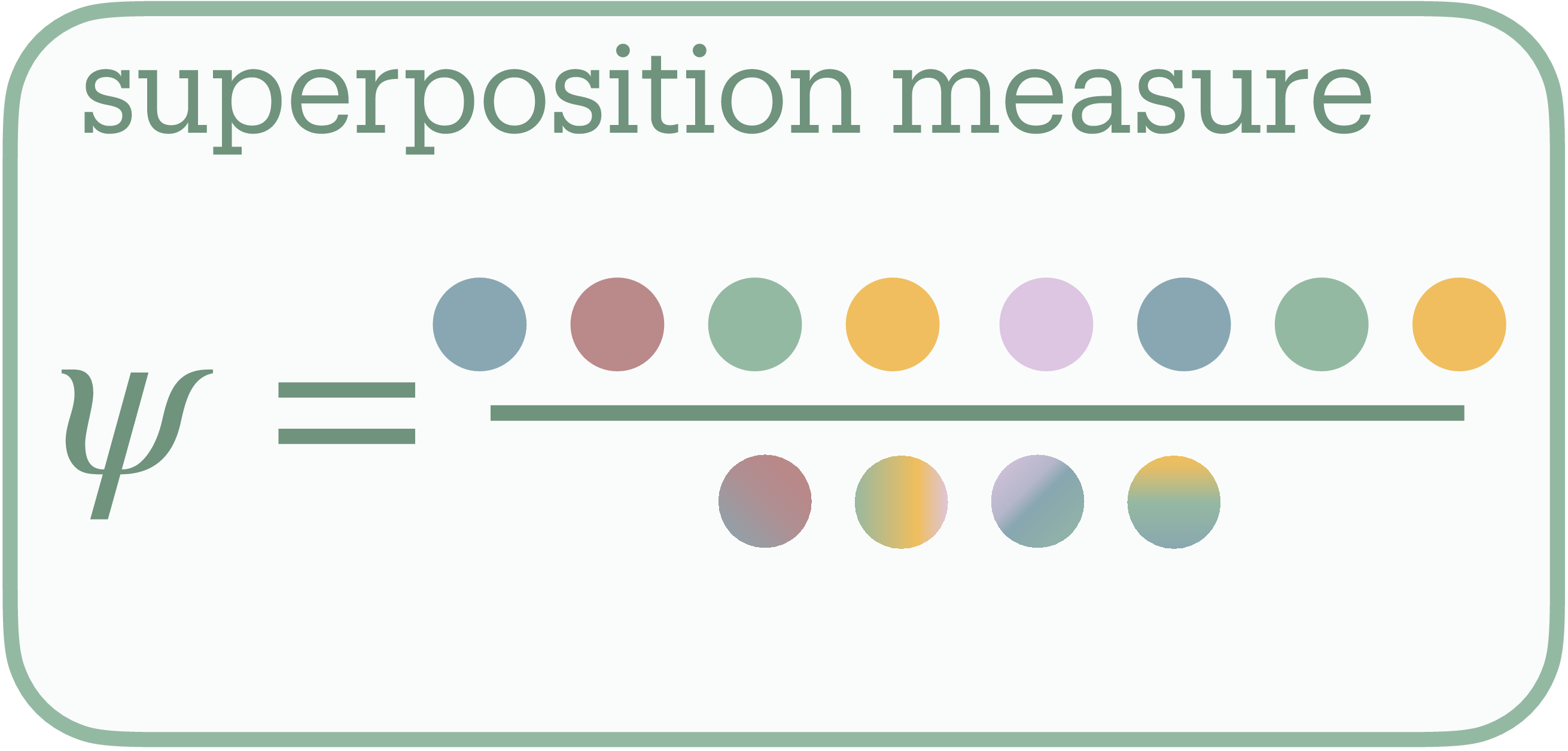
We measure superposition as $\psi = F/N$ (Figure 2c), counting virtual neurons per physical neuron. At $\psi = 1$, the network operates at its interference-free limit (no superposition). At $\psi = 2$, it simulates twice as many channels as it has neurons, achieving 2× lossy compression. Thus, we define superposition as compression beyond the lossless limit.

Our findings contradict the simple superposition-vulnerability hypothesis. Adversarial training does not universally reduce superposition; its effect depends on task complexity relative to network capacity (Section 7). Simple tasks with ample capacity permit abundance: networks expand features for robustness. Complex tasks under constraints force scarcity: networks compress further, reducing features. This bifurcation holds across architectures (MLPs, CNNs, ResNet-18) and datasets (MNIST, Fashion-MNIST, CIFAR-10).
We validate the framework where superposition is observable. Toy models achieve $r = 0.94$ correlation through the SAE extraction pipeline (Section 5.1), and under SAE dictionary scaling the measure converges with appropriate regularization (Section 5.2). Beyond adversarial training, systematic measurement across contexts generates hypotheses about neural organization: dropout seems to act as capacity constraint, reducing superposition (Section 6.1), compressing networks trained on algorithmic tasks seems to not create superposition ($\psi \leq 1$) likely due to lack of input sparsity (Section 6.2), during grokking, we capture the moment of algorithmic discovery through sharp drop in superposition at the generalization transition (Section 6.3), and Pythia-70M’s layer-wise compression peaks in early MLPs before declining (Section 6.4); mirroring intrinsic dimensionality studies
This work makes superposition measurable. By grounding neural compression in information theory, we enable quantitative study of how networks encode information under capacity constraints, potentially enabling systematic engineering of interpretable architectures.
Related Work
Superposition and polysemanticity
Neural networks employ distributed representations, encoding information across multiple units rather than in isolated neurons
While superposition (more effective features than neurons) inevitably creates polysemantic neurons through feature interference, polysemanticity (multiple features sharing a neuron) also emerges by other means: rotation of features relative to the neuron basis, incidentally
Sparse autoencoders for feature extraction
Sparse autoencoders (SAEs) tackle the challenge of extracting interpretable features from polysemantic representations by recasting it as sparse dictionary learning
SAEs scale to state-of-the-art models: Anthropic extracted millions of interpretable features from Claude 3 Sonnet
Information theory and neural measurement
Information-theoretic principles provide rigorous foundations for understanding neural representations. The information bottleneck principle
Most pertinent to our work, Ayonrinde et al.
Quantifying feature entanglement
Despite its theoretical importance, measuring superposition remains unexplored. Elhage et al.
Entropy-based measures have proven effective across disciplines facing similar measurement challenges. Neuroscience employs participation ratios (form of entropy, see Appendix for connection to Hill numbers) to quantify how many neurons contribute to population dynamics
Background on Superposition and Sparse Autoencoders
Neural networks must transmit information through layers with fixed dimensions. When neurons must encode information about many more features than available dimensions, networks employ superposition: packing multiple features into shared dimensions through interference. This compression mechanism enables representing more features than available neurons at the cost of introducing crosstalk between them. Superposition is compression beyond the lossless limit.
We examine toy models where superposition emerges under controlled bandwidth constraints, making interference patterns directly observable (Section 3.1). For real networks where ground truth remains unknown, we extract features through sparse autoencoders before measurement becomes possible (Section 3.2).
Observing Superposition in Toy Models
To understand how neural networks represent more features than they have dimensions, Elhage et al.
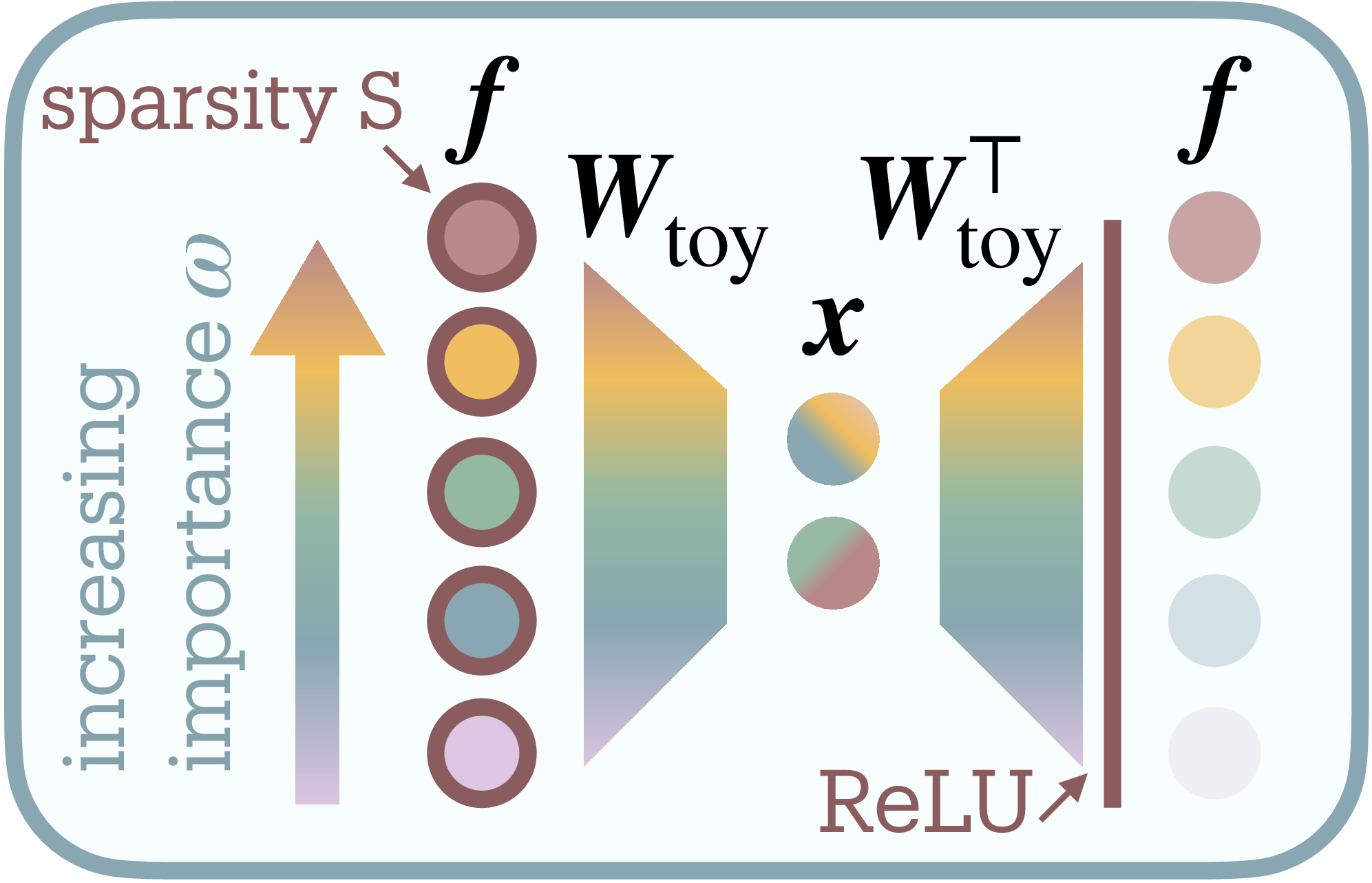
Here $M$ counts input features, $N$ counts bottleneck neurons, and $\mathbf{W}_{\text{toy}} \in \mathbb{R}^{N \times M}$ maps between them. The model must represent $M$ features using only $N$ dimensions; impossible unless features share neuronal resources.
Each input feature $f_i$ samples uniformly from $[0,1]$ with sparsity $S$ (probability of being zero) and importance weight $\omega_i$. Training minimizes importance-weighted reconstruction error $\mathcal{L}(\mathbf{f}) = \sum_{i=1}^M \omega_i|f_i - f’_i|^2$, revealing how networks optimally allocate limited bandwidth.
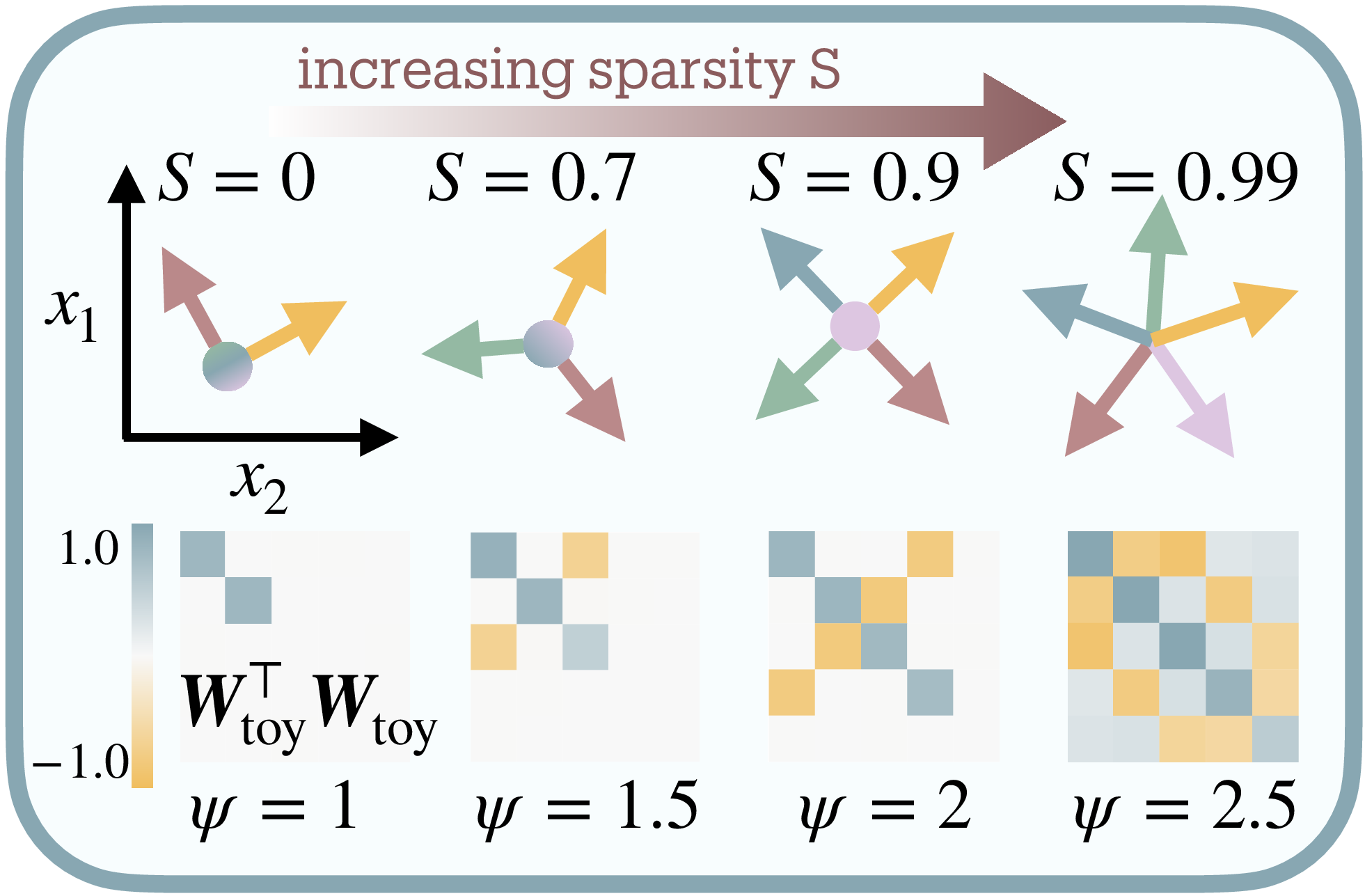
As sparsity increases, the model packs features into shared dimensions through nearly-orthogonal arrangements (Figure 2b). The interference matrix $\mathbf{W}_{\text{toy}}^T \mathbf{W}_{\text{toy}}$ reveals this geometric solution: at low compression, strong diagonal with minimal off-diagonal terms; at high compression, substantial off-diagonal interference as features share space. These interference terms quantify the distortion networks accept for increased capacity. The ReLU nonlinearity proves essential, suppressing small interference to maintain reconstruction despite feature overlap.
Elhage et al.
This weight-based approach requires knowing the true feature-to-neuron mapping (unavailable in real networks) and lacks scale invariance; multiplying weights by any constant arbitrarily changes the measure. We need a principled framework quantifying compression without ground truth features.
Extracting Features Through Sparse Autoencoders
Real networks do not reveal their features directly. Instead, we must untangle them from distributed neural activations. Sparse autoencoders (SAEs) decompose activations into sparse combinations of learned dictionary elements, effectively reverse-engineering the toy model’s feature representation
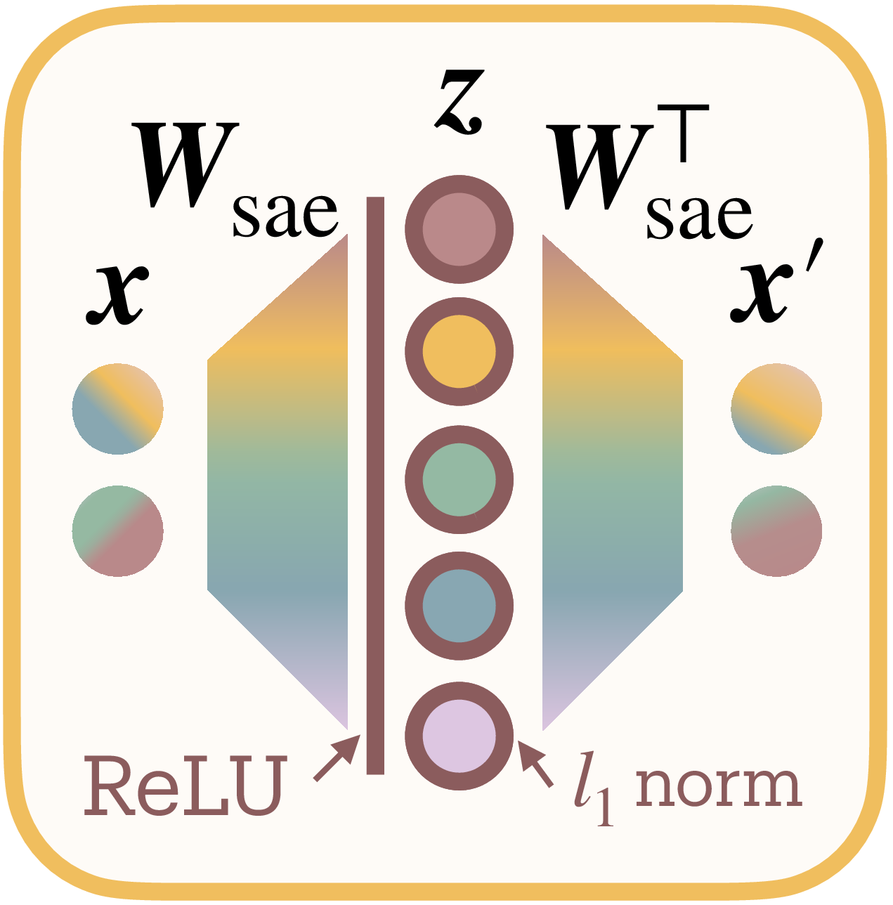
Given layer activations $\mathbf{x} \in \mathbb{R}^N$, an SAE learns a higher-dimensional sparse code $\mathbf{z} \in \mathbb{R}^D$ where $D > N$ (Figure 2c):
The reconstruction combines these sparse features:
where columns $\mathbf{d}_i$ of $\mathbf{W}_{\text{dec}}$ form the learned dictionary.
Training balances faithful reconstruction against sparse activation:
The $\ell_1$ penalty creates explicit competition: the bound on total activation $\sum_i \lvert z_i\rvert$ forces features to justify their magnitude by contributing to reconstruction. This implements resource allocation where larger $\lvert z_i\rvert$ indicates greater consumption of the network’s limited representational budget (see Appendix for rate-distortion derivation).
SAE design choices. We tie encoder and decoder weights ($\mathbf{W}_{\text{dec}} = \mathbf{W}_{\text{enc}}^T$) to enforce features as directions in activation space, maintaining conceptual clarity at potential cost to reconstruction
If networks truly employ superposition, SAEs should recover the underlying features enabling measurement. Recent work shows SAE features causally affect network behavior
Measuring Superposition Through Information Theory
We quantify superposition by determining how many neurons would be required to transmit the observed feature distribution without interference. Information theory provides a precise answer: Shannon’s source coding theorem establishes that any distribution with entropy $H(p)$ can be losslessly compressed to $e^{H(p)}$ uniformly-allocated channels. This represents the minimum bandwidth for interference-free transmission; the network’s effective degrees of freedom.
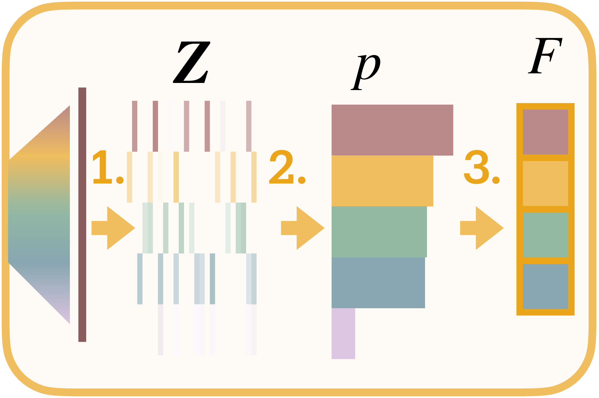
We formalize superposition as the compression ratio $\psi = F/N$, where $N$ counts physical neurons and $F = e^{H(p)}$ measures effective degrees of freedom extracted from SAE activation statistics1 (Figure 2d). When $\psi = 1$, the network operates at the lossless boundary. When $\psi > 1$, features necessarily share dimensions through interference. For instance, in Figure 2b, 5 features represented in 2 neurons yields $\psi = 2.5$.
Feature probabilities from resource allocation. Consider a layer with $N$ neurons whose activations have been processed by an SAE with dictionary size $D$. Across $S$ samples, the SAE produces sparse codes $\mathbf{Z} = \text{ReLU}(\mathbf{W}_{\text{sae}}\mathbf{X}) \in \mathbb{R}^{D \times S}$ where $\mathbf{X} \in \mathbb{R}^{N \times S}$ contains the original activations. Each feature’s probability reflects its share of total activation magnitude2:
The SAE’s $\ell_1$ regularization ensures these allocations reflect computational importance. Features activating more frequently or strongly consume more capacity, with optimal $\lvert z_i\rvert$ proportional to marginal contribution to reconstruction quality (derivation in Appendix).
Effective features as lossless compression limit. Shannon entropy quantifies the information content of this distribution $H(p) = -\sum_i p_i \log p_i$. Its exponential:
measures effective degrees of freedom, the minimum neurons needed to encode $p$ without interference. This is the network’s lossless compression limit: the feature distribution could be transmitted through $F$ neurons with no information loss. Using fewer than $F$ neurons guarantees interference as features must share dimensions; using exactly $F$ achieves the interference-free boundary. The actual layer width $N$ determines whether compression remains lossless ($N \geq F$) or becomes lossy ($N < F$). The ratio then measures superposition as lossy compression:
While the SAE extracts $D$ interpretable features, semantic concepts humans might recognize, our measure quantifies $F$ effective features, the interference-free channel capacity required for their activation distribution. A network might use $D=1000$ interpretable features but need only $F=50$ effective features if most activate rarely.
Our measure inherits desirable properties from entropy. First, for any $D$-component distribution, the output stays bounded: $1 \leq F(p) \leq D$, constrained by single-feature dominance and uniform distribution. Second, unlike threshold-based counting, features contribute according to their information content: rare features matter less than common ones; weak features less than strong ones. This enables the interpretation as effective degrees of freedom, beyond merely “counting features.”
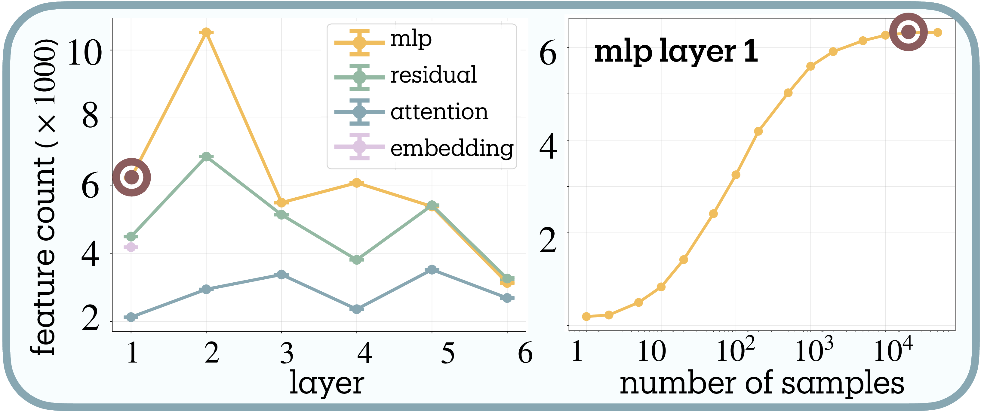
In practice, we use sufficient samples until convergence (see convergence analysis in Section 6.4). For convolutional layers, we treat spatial positions as independent samples, measuring superposition across the channel dimension (see Appendix). While the data distribution for extracting SAE activations should generally reflect the training distribution, for studying adversarial training’s effect, we evaluate on both clean inputs and adversarially perturbed inputs for contrast.
This framework enables quantifying superposition without ground truth by measuring each layer’s compression ratio; how many virtual neurons it simulates relative to its physical dimension.
Validation of the Measurement Framework
Toy Model of Superposition
We validate our measure using the toy model of superposition
Following Elhage et al.
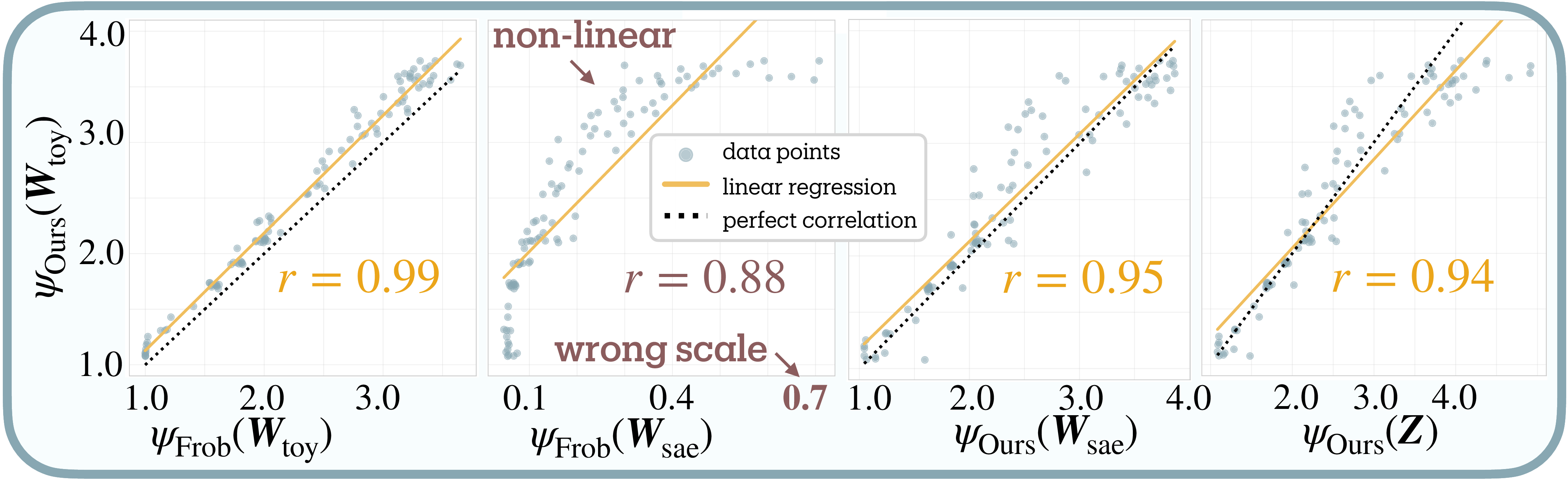
Validation strategy. Our validation proceeds in two steps. First, we establish reference values by measuring superposition directly from $\mathbf{W}_{\text{toy}}$, where the interference matrix $\mathbf{W}_{\text{toy}}^T \mathbf{W}_{\text{toy}}$ reveals compression levels: diagonal dominance indicates orthogonal features; off-diagonal terms show interference (Figure 2b). Both our entropy-based measure and the Frobenius norm baseline (Equation 2) achieve near-perfect correlation ($r = 0.99 \pm 0.01$) when applied to toy model weights, confirming both track these observable patterns (Figure 3a).
Second, we test whether each metric recovers these reference values when given only SAE outputs, the realistic scenario for measuring real networks. Here the Frobenius norm fails catastrophically on SAE weights, producing nonlinear relationships and incorrect scales (0.1–0.7 versus expected 1–4); the $\ell_1$ regularization fundamentally alters weight statistics. Our activation-based approach maintains strong correlation ($r = 0.94 \pm 0.02$) with the reference values even through the SAE bottleneck.
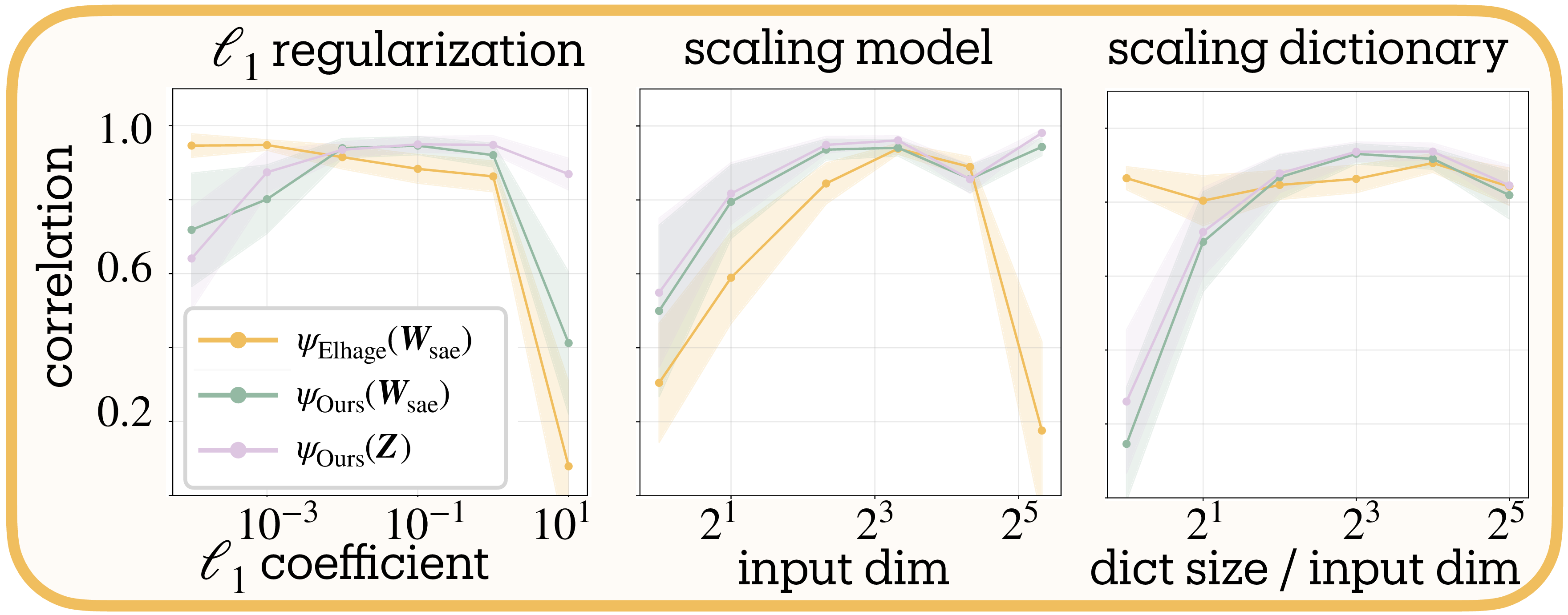
Hyperparameter stability. We test sensitivity across three axes: $\ell_1$ strength ($10^{-3}$ to $10^1$), model scale (8–32 input dimensions), and dictionary expansion (2× to 32×). Figure 3b shows stable performance across most configurations. Correlation degrades when extreme regularization ($\ell_1 = 10$) suppresses features, when dictionaries lack capacity to represent the feature set, when toy models are too small or too large to train reliably, or when very large dictionaries enable feature splitting (see Section 5.2). These failure modes reflect limitations of the toy model or SAE training rather than the measure itself.
Dictionary Scaling Convergence
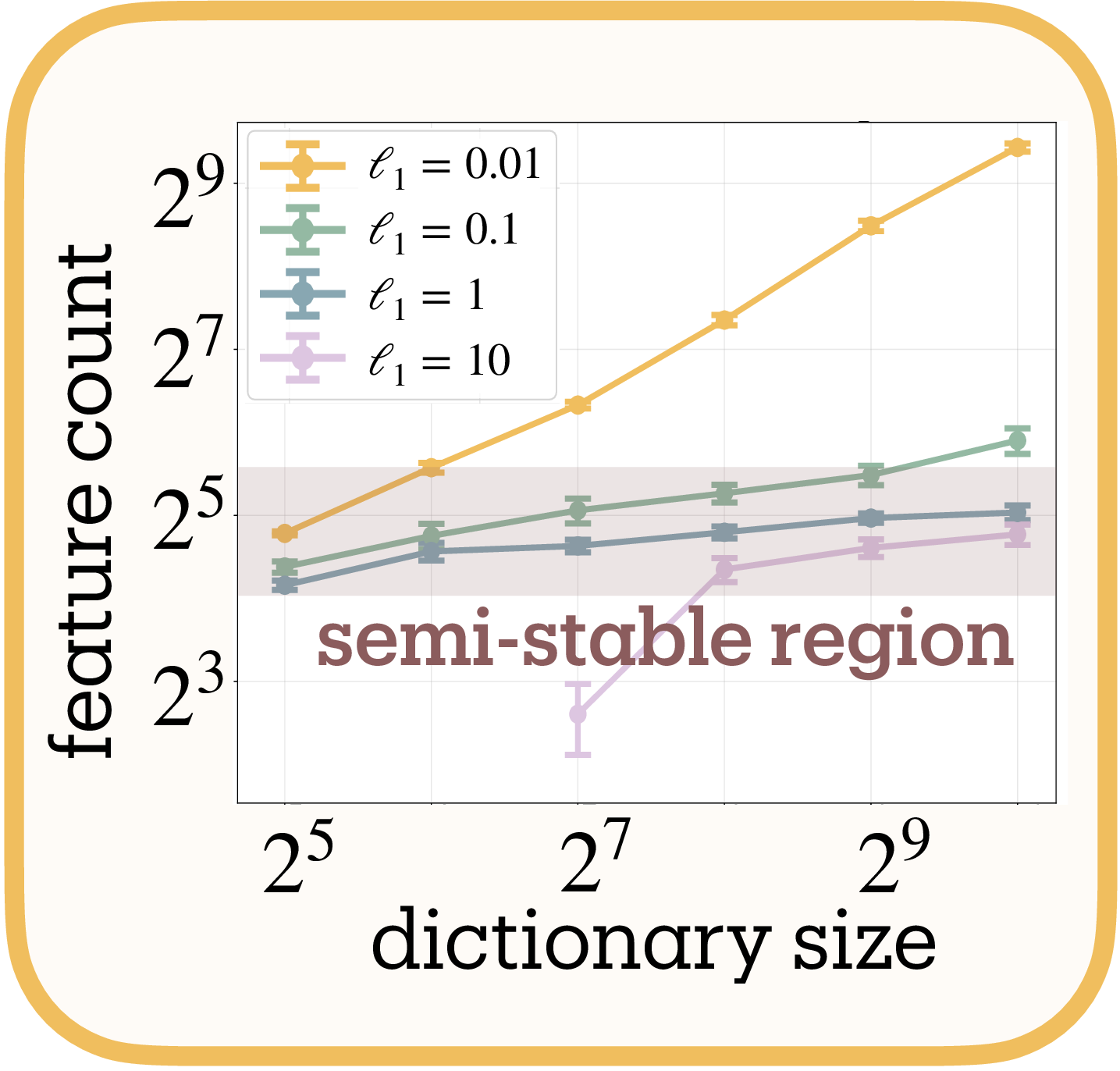
Measuring a natural coastline with a finer ruler yields a longer measurement; potentially without bound
We test convergence using multi-task sparse parity
Figure 4a reveals two regimes. With appropriate regularization ($\ell_1 \geq 0.1$), feature counts plateau despite dictionary expansion, indicating we measure the network’s representational structure and not arbitrary decomposition; i.e. feature splitting
The dependence on dictionary size means absolute counts vary with SAE architecture, but comparative measurements remain valid: networks analyzed under identical configurations yield meaningful relative differences, even as changing those configurations shifts all measurements systematically.
Applications and Findings
We measure superposition across four neural compression phenomena: capacity constraint under dropout (Section 6.1), algorithmic tasks that resist superposition despite compression (Section 6.2), developmental dynamics during learning transitions (Section 6.3), and layer-wise representational organization in language models (Section 6.4).
Each finding here is a preliminary, exploratory analysis on specific architectures and tasks. Our primary contribution remains the measurement tool itself. These findings illustrate its potential utility while generating testable hypotheses for future systematic investigation across broader experimental conditions.
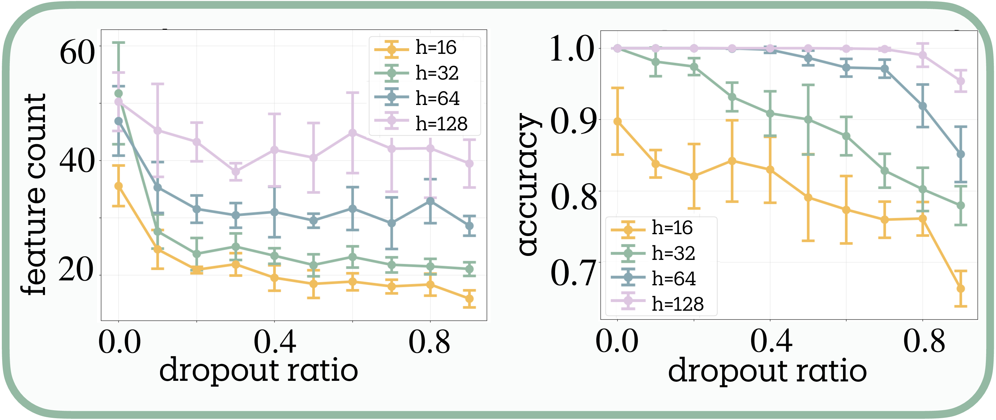
Dropout Reduces Features Through Redundant Encoding
We investigate how dropout affects feature organization using multi-task sparse parity (3 tasks, 4 bits each) with simple MLPs across hidden dimensions $h \in {16, 32, 64, 128}$ and dropout rates [0.0, 0.1, …, 0.9].
Marshall et al.
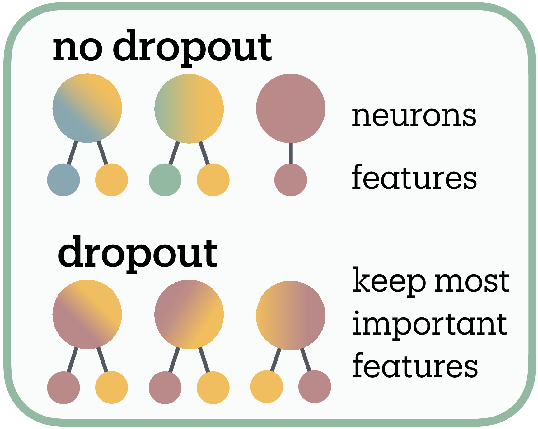
We propose this reflects the distinction between polysemanticity and superposition (Figure 4c). If dropout forces each feature to occupy multiple neurons for robustness, this redundant encoding would consume capacity, leaving room for fewer total features within the same dimensional budget. Under this interpretation, networks respond by pruning less essential features, consistent with Scherlis et al.’s
The capacity dependence supports this account: larger networks show reduced dropout sensitivity while narrow networks exhibit sharp feature reduction, suggesting capacity constraints mediate the effect.
Algorithmic Tasks Resist Superposition Despite Compression
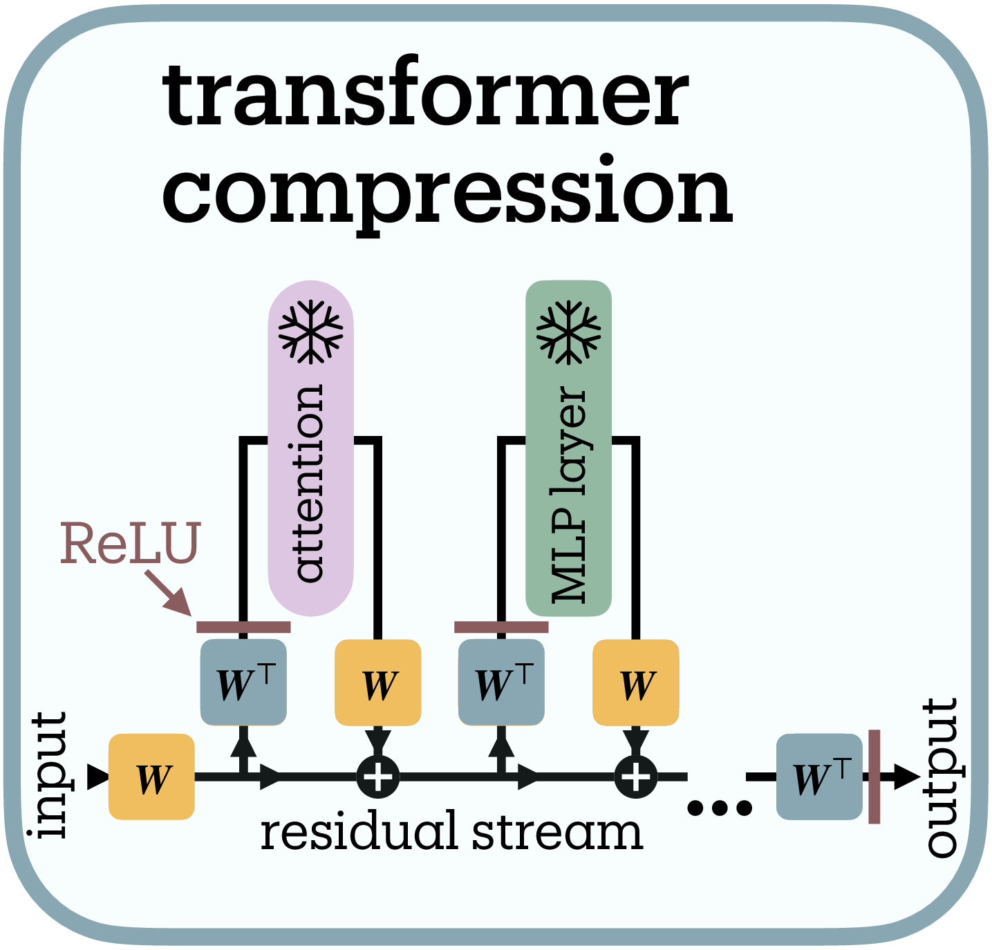
Tracr compiles human-readable programs into transformer weights with known computational structure
Following Lindner et al.
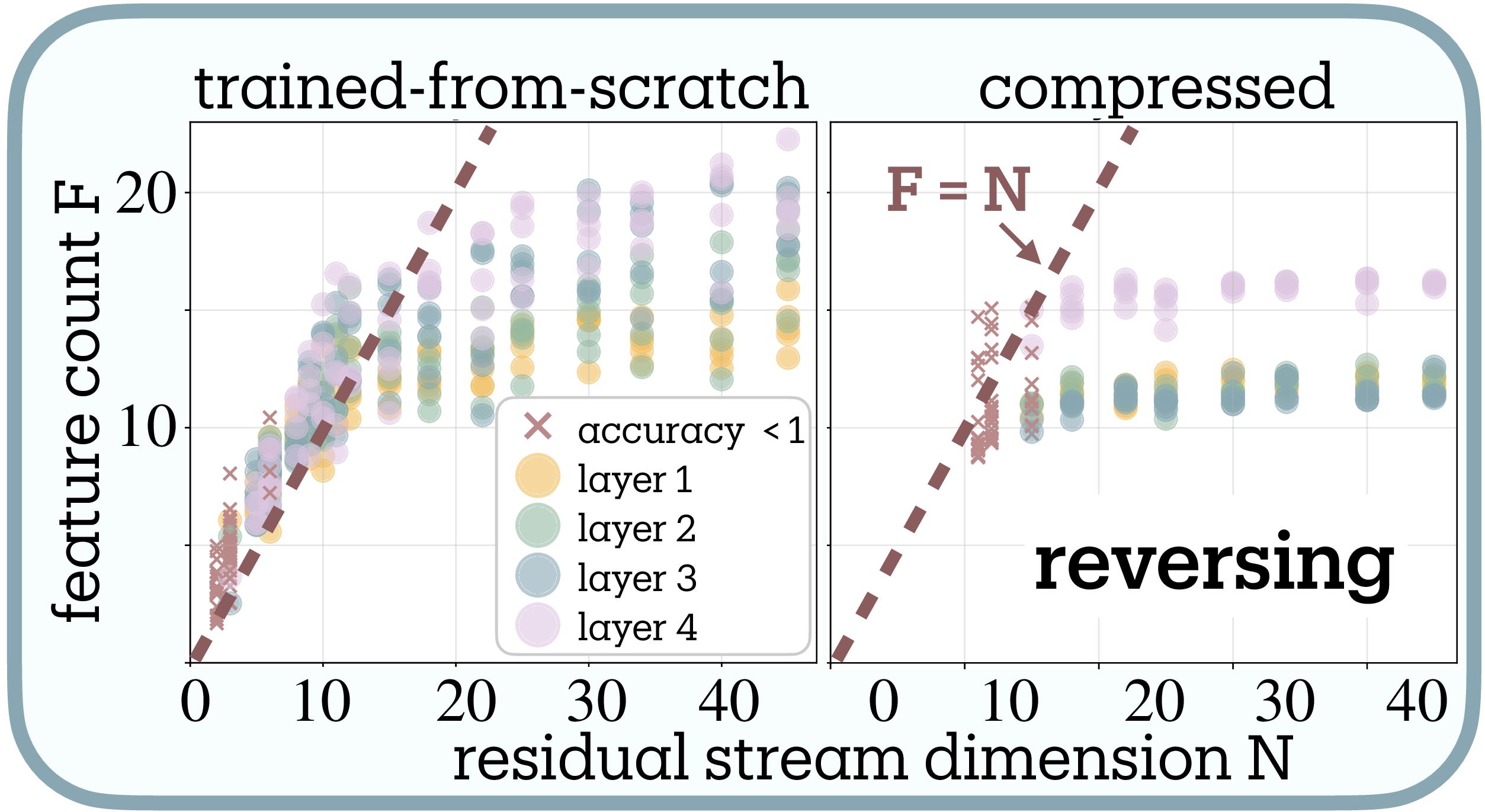
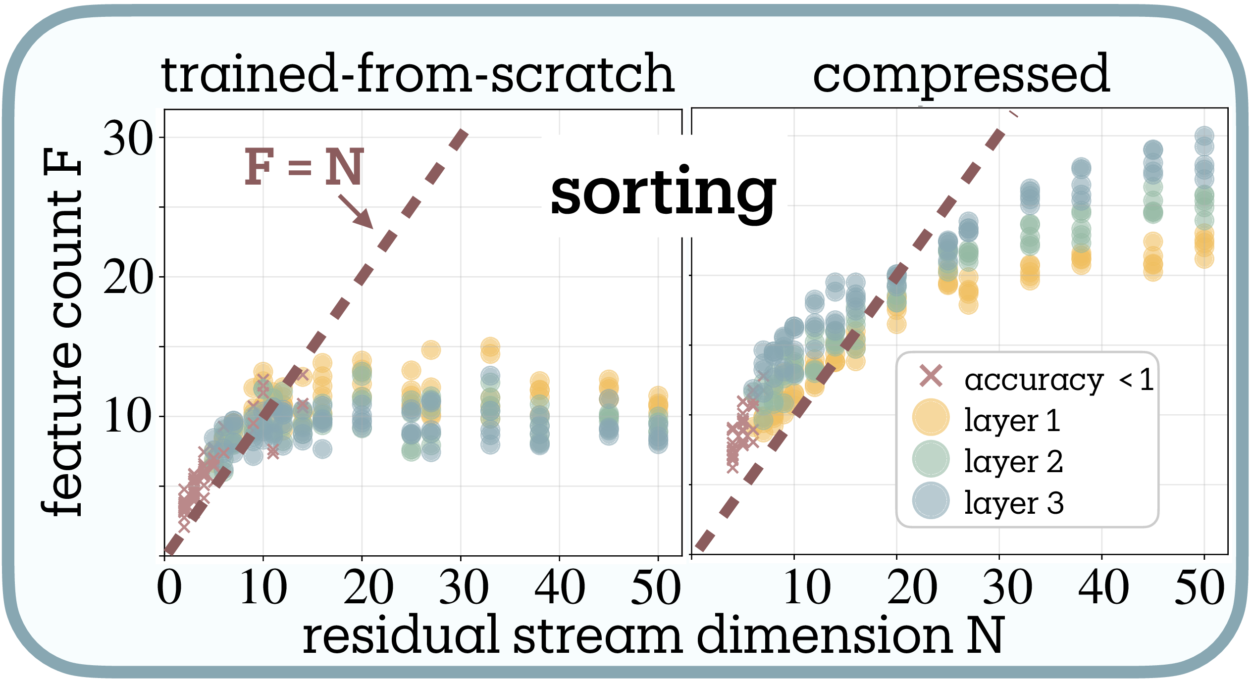
The compression dynamics reveal limits on superposition in these algorithmic tasks (Figure 5b, 5c). Both compiled Tracr models and transformers trained from scratch converge to ~12 features for reversal and ~10 for sorting3—far below their original compiled dimensions (45D for reversal), revealing substantial dimensional redundancy in Tracr’s compilation.
As compression reduces dimensions from 45D toward the task-intrinsic boundary, superposition increases from $\psi \approx 0.3$ toward $\psi = 1$. However, compression stops increasing superposition once models reach the $F=N$ diagonal: further dimensional reduction causes linear drop in effective features and eventually performance collapse (× markers) rather than superposition beyond $\psi = 1$, resisting genuine superposition ($\psi > 1$) entirely.
This resistance likely stems from algorithmic tasks violating the sparsity assumption required for lossy compression
Capturing Grokking Phase Transition
Grokking (sudden perfect generalization after extended training on algorithmic tasks) provides an ideal testbed for developmental measurement
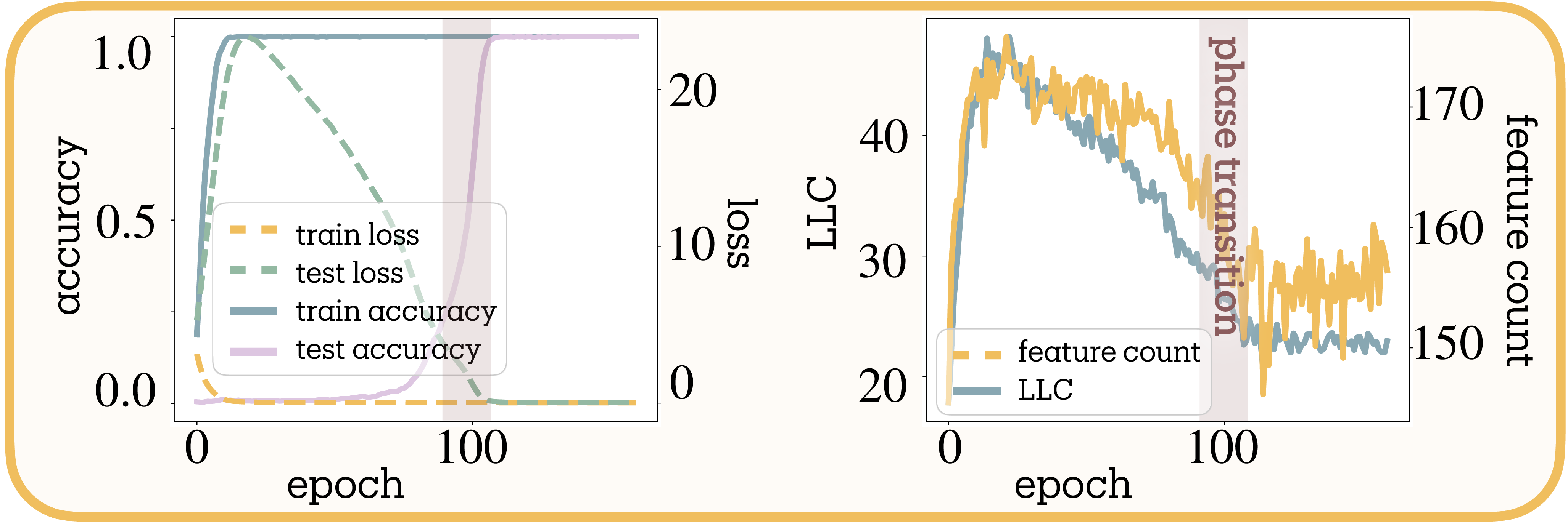
We train a two-path MLP on modular arithmetic $(a + b) \bmod 53$. Figure 6b reveals distinct dynamics: while LLC shows initial proliferation followed by smooth decay throughout training, our feature count exhibits sharp consolidation precisely at the generalization transition.
This pattern suggests the measures capture different aspects of complexity evolution. During memorization, the model employs numerous superposed features to store input-output mappings. The sharp consolidation coincides with algorithmic discovery, where the model reorganizes from distributed lookup tables into compact representations that capture the modular arithmetic rule
Layer-wise Organization in Language Models
We analyze Pythia-70M using pretrained SAEs from Marks et al.
MLPs store the most features, followed by residual streams, with attention maintaining minimal counts, consistent with MLPs as knowledge stores and attention as routing
This non-monotonic trajectory parallels intrinsic dimensionality studies
Connection between Superposition and Adversarial Robustness
Testing the superposition-vulnerability hypothesis. The superposition-vulnerability hypothesis proposed by Elhage et al.
We employ PGD adversarial training
Statistical methodology. To quantify adversarial training effects, we extract normalized slopes representing how feature counts change per unit increase in adversarial training strength ($\epsilon \in {0.0, 0.1, 0.2, 0.3}$). Positive slopes indicate adversarial training increases features; negative slopes indicate reduction. For each experimental condition, we fit linear regressions to feature counts across epsilon values, pooling clean and adversarial observations to increase statistical power. These slopes are normalized by baseline ($\epsilon = 0$) feature counts, making effects comparable across layers with different absolute scales.
Since networks contain multiple layers, we aggregate layer-wise measurements using parameter-weighted averaging, where layers with more parameters receive proportionally higher weight. This reflects the assumption that computationally intensive layers better represent overall network behavior. For simple architectures, parameter counts include all weights and biases; for ResNet-18, we implement detailed counting that accounts for convolutions, batch normalization, and skip connections.
Testing Adversarial Training Effects on Superposition
- H1 (Universal Reduction): Adversarial training uniformly reduces superposition across all conditions, directly testing Elhage et al.'s original prediction.
- H2 (Complexity ↓): Higher task complexity shifts adversarial training's effect from feature expansion toward reduction. We encode complexity ordinally (2-class=1, 3-class=2, 5-class=3, 10-class=4) and test for negative linear trends in the adversarial training slope.
- H3 (Capacity ↑): Higher network capacity shifts adversarial training's effect from feature reduction toward expansion. We test for positive log-linear relationships between capacity measures and adversarial training slopes.
All statistical tests use inverse-variance weighting to account for measurement uncertainty, with random-effects meta-analysis when significant heterogeneity exists across conditions.
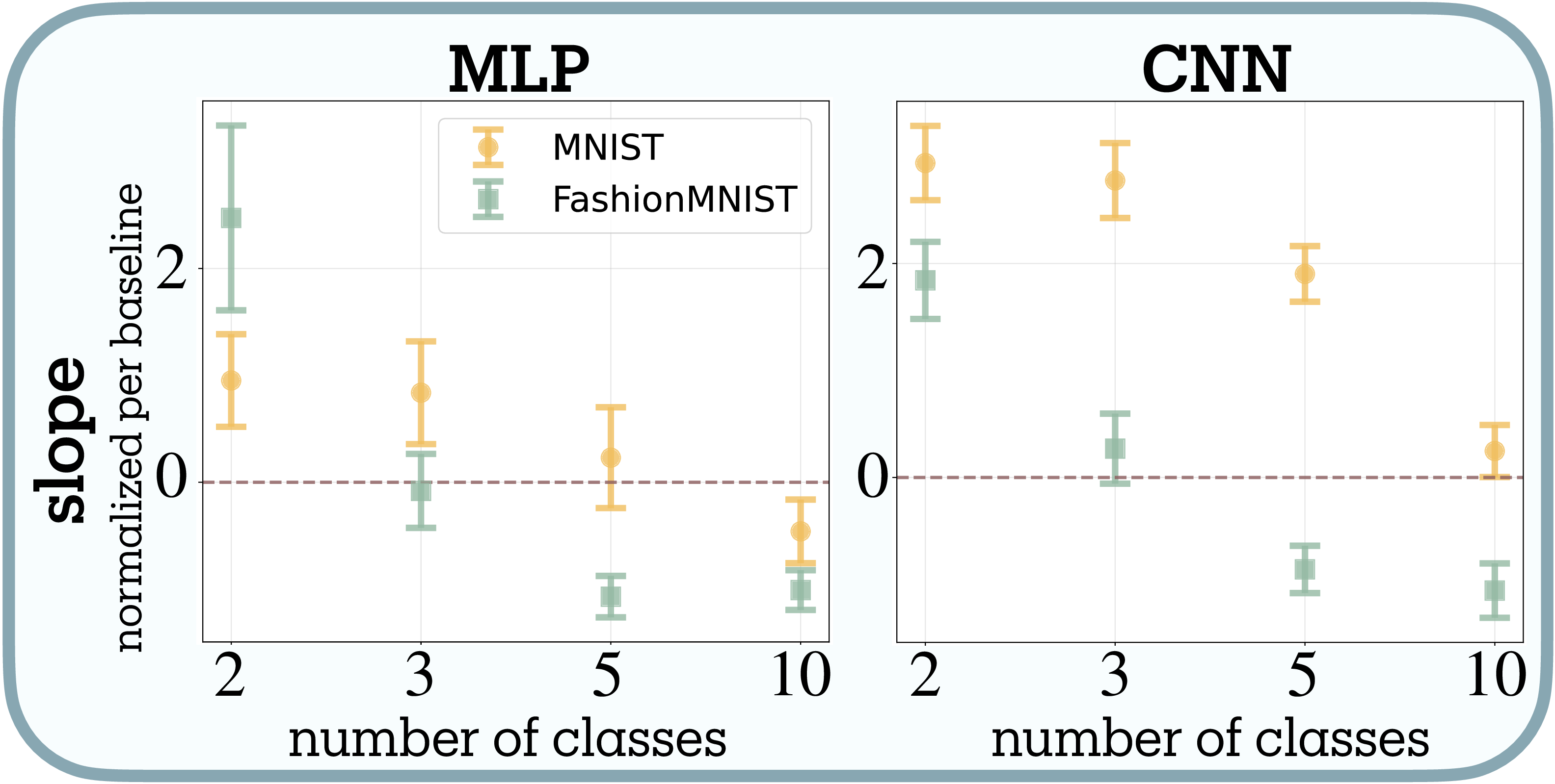
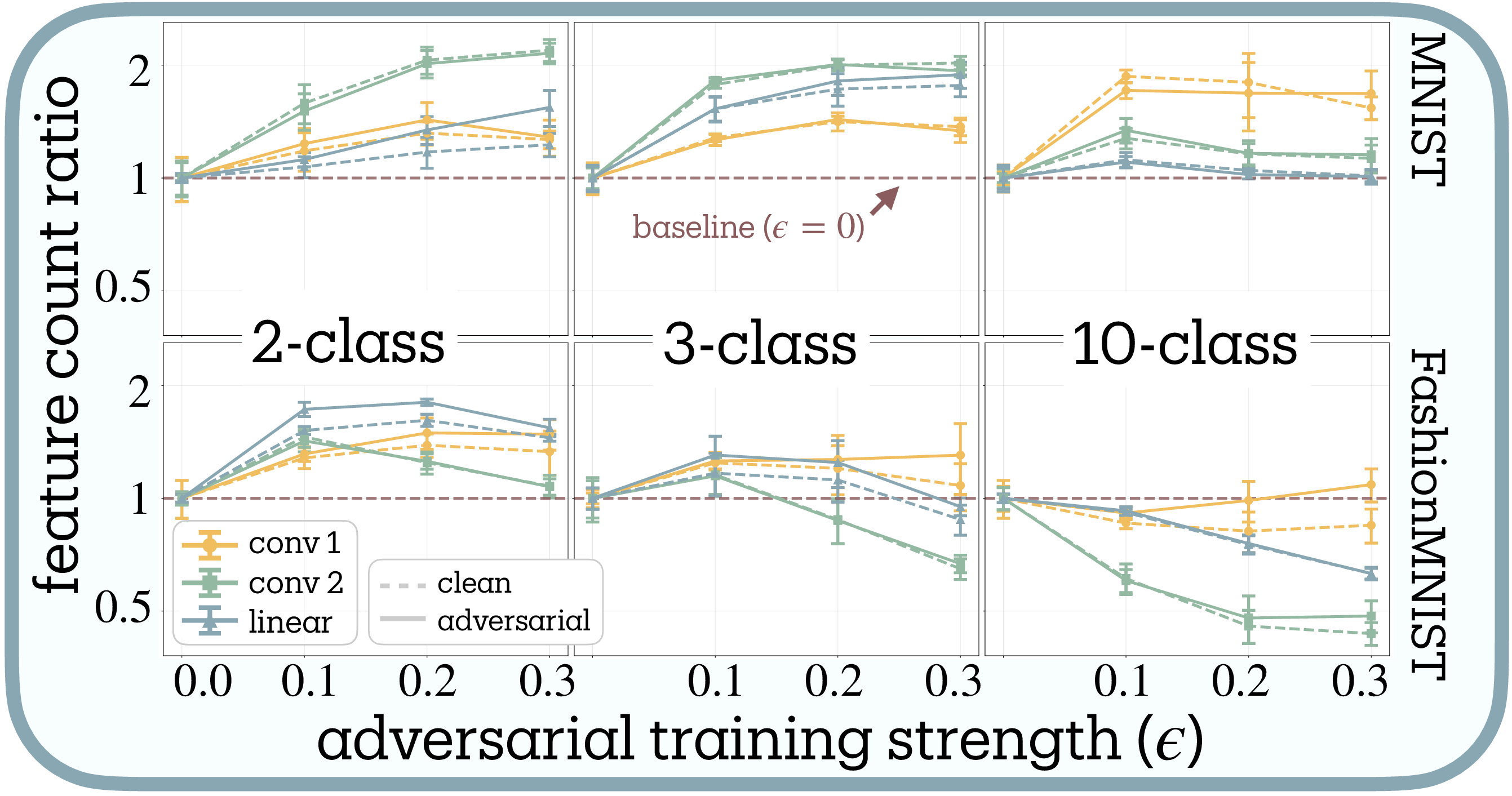
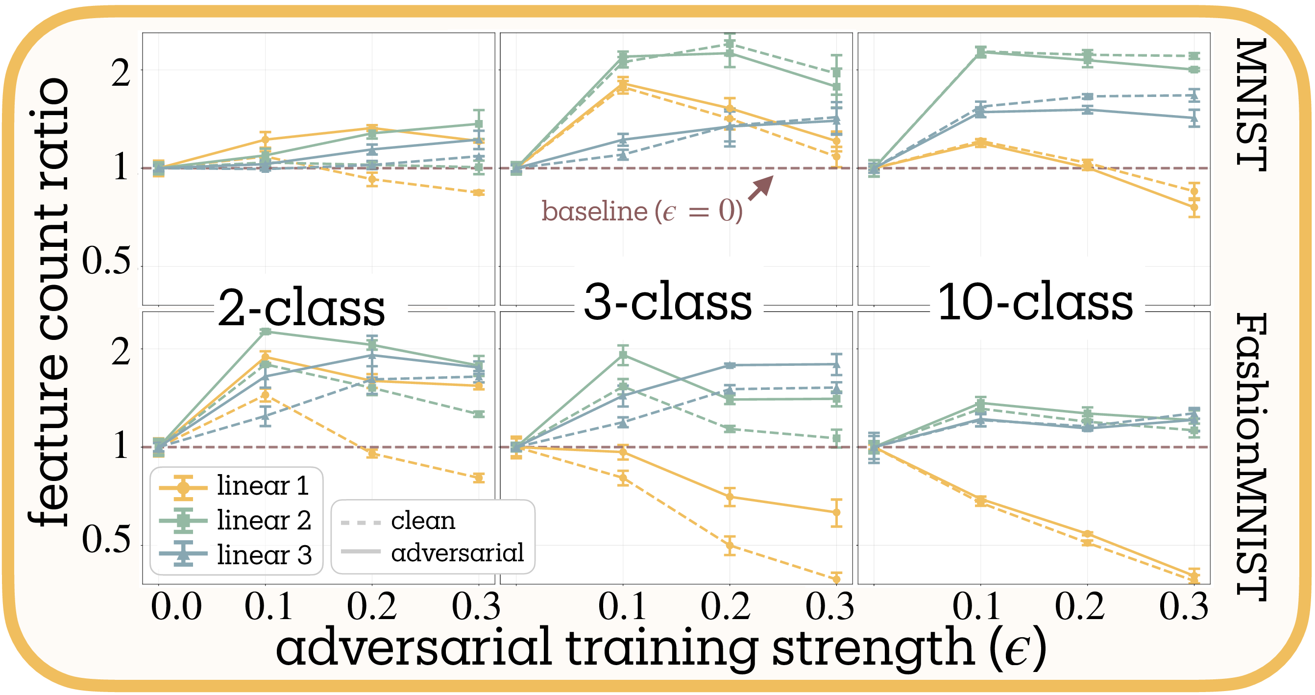
Complexity shifts adversarial training toward feature reduction (H2 supported). Contrary to H1’s prediction of universal reduction, adversarial training produces bidirectional effects whose direction depends systematically on task complexity (Figure 7 and Figure 9a). Our meta-analysis reveals significant heterogeneity across conditions ($Q = 8.047$, $df = 3$, $p = 0.045$), necessitating random-effects modeling. The combined effect confirms H2: a negative relationship between task complexity and the adversarial training slope (slope $= -0.745 \pm 0.122$, $z = -6.14$, $p < 0.001$), meaning higher complexity shifts the effect from expansion toward reduction.
Binary classification consistently yields positive slopes, with feature counts expanding up to 2× baseline. Networks appear to develop additional defensive features when task demands are simple. Ten-class problems show negative slopes, with feature counts decreasing by up to 60%, particularly in early layers. Three-class tasks exhibit intermediate behavior with inverted-U curves: moderate adversarial training ($\epsilon = 0.1$) initially expands features before stronger training ($\epsilon = 0.3$) triggers reduction.
Dataset difficulty amplifies these effects. Fashion-MNIST produces systematically more negative slopes than MNIST (mean difference $= -1.467 \pm 0.156$, $t(7) = -2.405$, $p = 0.047$, Cohen’s $d = -0.85$), consistent with its design as a more challenging benchmark
Layer-wise patterns differ between architectures: MLP first layers reduce most while CNN second layers reduce most. We lack a mechanistic explanation for this divergence.
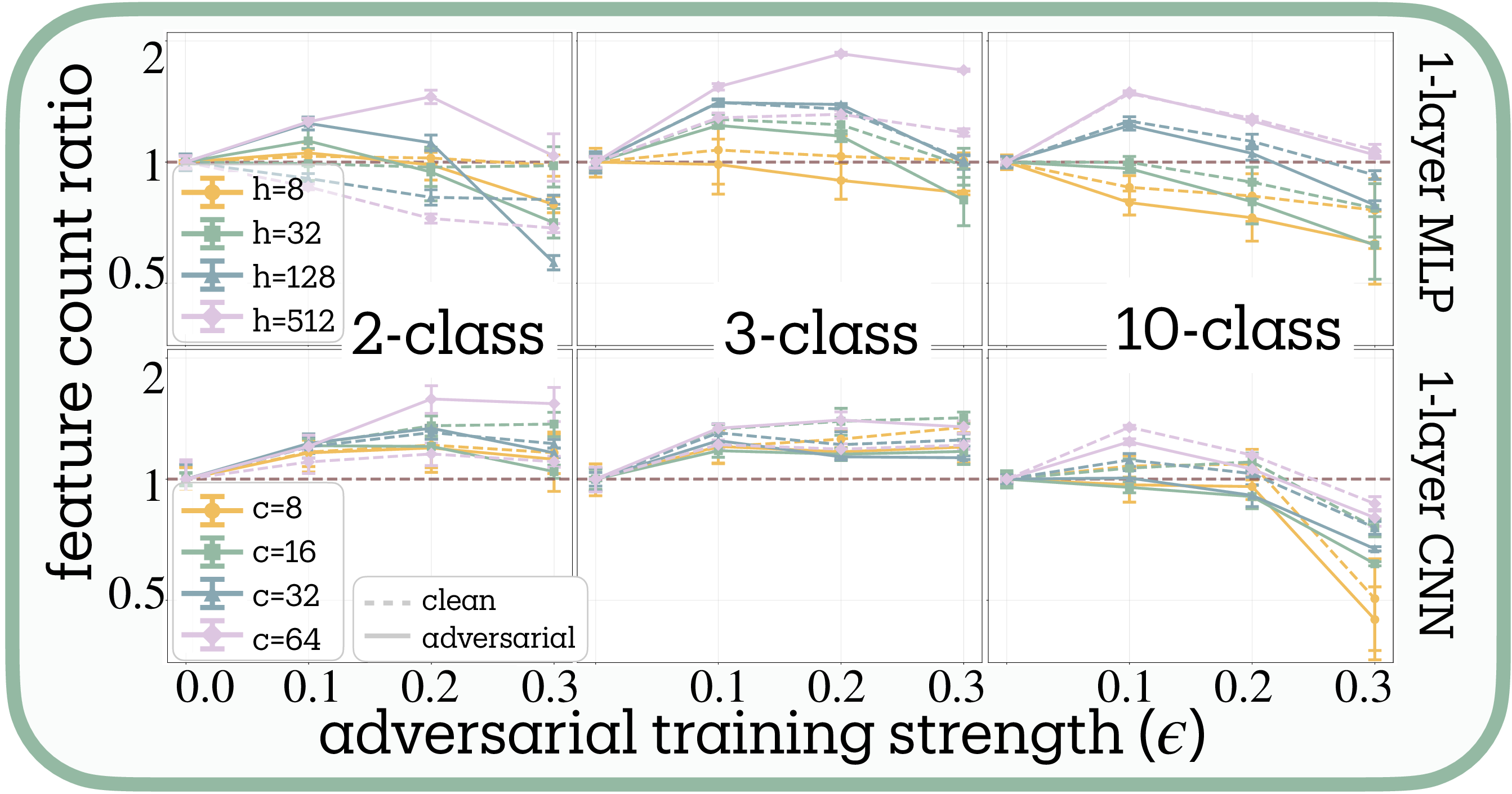
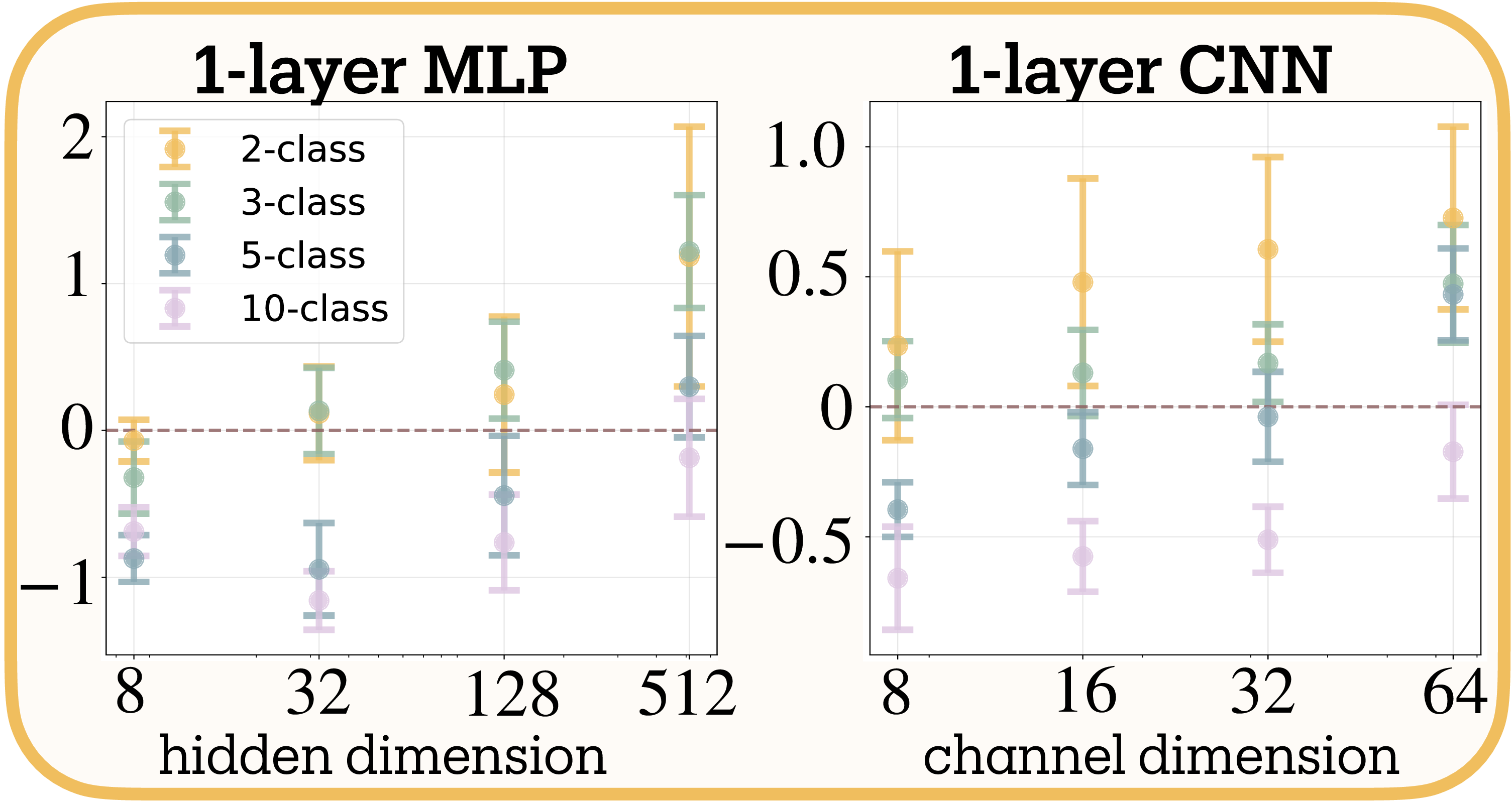
Capacity shifts adversarial training toward feature expansion (H3 supported). Network capacity exhibits a positive relationship with the adversarial training slope, strongly supporting H3 (Figure 8, Figure 9b, 9c). Single-layer networks demonstrate clear capacity thresholds (meta-analytic slope $= 0.220 \pm 0.037$, $z = 5.90$, $p < 0.001$). Networks with minimal capacity (8 hidden units for MLPs, 8 filters for CNNs) show negative slopes—reducing features across all task complexities—while high-capacity networks (512 units/64 filters) show positive slopes, expanding features even for 10-class problems.
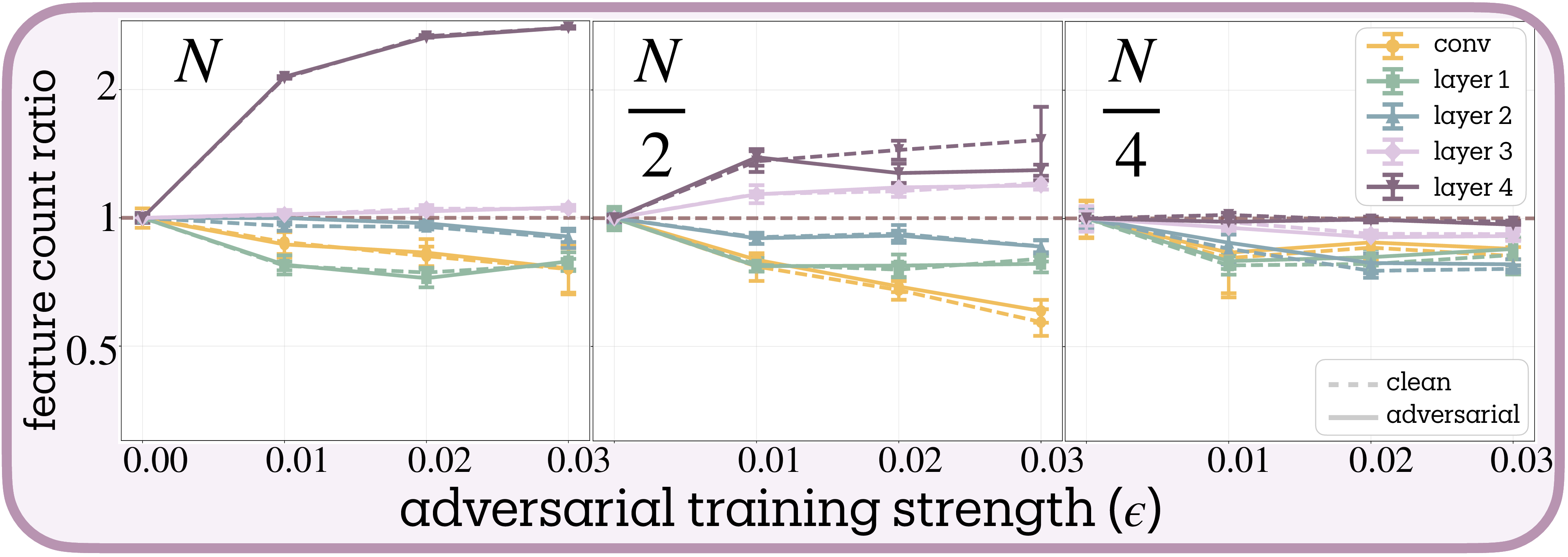
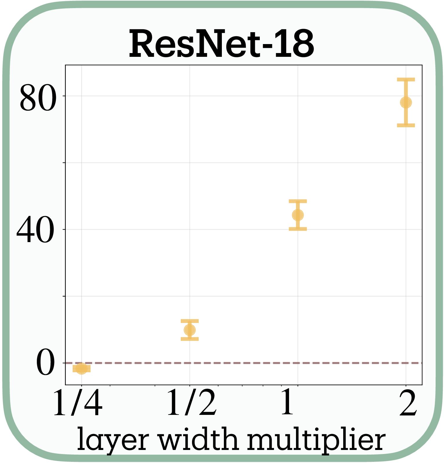
This capacity dependence scales dramatically in deep architectures. ResNet-18 on CIFAR-10 exhibits a strong log-linear relationship between width multiplier and adversarial training slopes (slope $= 31.0 \pm 2.0$ per $\log(\text{width})$, $t(2) = 15.7$, $p = 0.004$, $R^2 = 0.929$). An 8-fold width increase (0.25× to 2×) produces a 65-unit change in normalized slope. At minimal width (0.25×), adversarial training barely affects feature counts; at double width, networks show massive feature expansion with slopes approaching 80.
The layer-wise progression in ResNet-18 reveals hierarchical specialization: early layers (conv1, layer1) reduce features by up to 50%, middle layers remain stable, while deep layers (layer3, layer4) expand up to 4×. Systematically narrowing the network dampens this pattern: at 1/4 width, late-layer expansion vanishes while early-layer reduction persists but weakens. This could reflect vulnerability hierarchies, where early layers processing low-level statistics are easily exploited by imperceptible perturbations, necessitating feature reduction, while late layers encoding semantic information can safely expand their representational repertoire.
Two regimes of adversarial response. Our findings reveal a more nuanced relationship between superposition and adversarial vulnerability than originally theorized. Rather than universal feature reduction, adversarial training operates in two distinct regimes determined by the ratio of task demands to network capacity.
Bifurcation Driven by Task Complexity to Network Capacity Ratio
- Abundance regime (low complexity / high capacity): Adversarial training increases effective features. Networks add defensive features, achieving robustness through elaboration.
- Scarcity regime (high complexity / low capacity): Adversarial training decreases effective features. Networks prune to fewer, potentially more orthogonal features, as predicted by the superposition-vulnerability hypothesis.
Unexplained patterns. Several patterns in our data remain unexplained. We observe non-monotonic inverted-U curves where moderate adversarial training ($\epsilon = 0.1$) expands features while stronger training ($\epsilon = 0.3$) reduces them below baseline. The gap between clean and adversarial feature counts varies unpredictably; sometimes negligible, sometimes substantial. Some results contradict our complexity hypothesis, with 2-class MLPs occasionally showing lower feature counts than 3-class. CNN experiments consistently yield stronger statistical significance ($p < 0.02$) than equivalent MLP experiments ($p \approx 0.09$) for unknown reasons.
Implications for interpretability. Our findings complicate simple accounts of why robust models often appear more interpretable
The bidirectional relationship between robustness and superposition suggests that achieving robustness without capability loss may require ensuring sufficient capacity for defensive elaboration. While our experiments demonstrate that increased robustness can coincide with either increased or decreased superposition depending on the regime, establishing the exact causal connection between superposition and robustness remains an important direction for future work.
Limitations
Our superposition measurement framework is limited by its dependence on sparse autoencoder quality, theoretical assumptions about neural feature representation, and should be interpreted as a proxy for representational complexity rather than a literal feature count.
Sparse autoencoder quality. Our approach inherently depends on sparse autoencoder feature extraction quality. While recent architectural advances (gated SAEs
Assumptions on feature representation. Our framework rests on several assumptions that real networks systematically violate. The linear representation assumption (that features correspond to directions in activation space) has been challenged by recent discoveries of circular feature organization for temporal concepts
Comparative rather than absolute count. Our measure quantifies effective representational diversity under specific assumptions rather than providing literal feature counts. This creates several interpretational limitations. The measure exhibits sensitivity to the activation distribution used for measurement. SAE training distributions must match the network’s operational regime to avoid systematic bias. Feature granularity remains fundamentally ambiguous: broader features may decompose into specific ones in wider SAEs, creating uncertainty about whether we’re discovering or creating features. Our single-layer analysis potentially misses features distributed across layers through residual connections or attention mechanisms. Most critically, we measure the effective alphabet size of the network’s internal communication channel rather than counting distinct computational primitives, making comparative rather than absolute interpretation most appropriate.
The limitations largely reflect active research areas in sparse dictionary learning and mechanistic interpretability. Each advance in SAE architectures, training procedures, or theoretical understanding directly benefits measurement quality. Within its scope—comparative analysis of representational complexity under sparse linear encoding assumptions—the measure enables systematic investigation of neural information structure previously impossible.
Future Work
Cross-model feature alignment. Following Anthropic’s crosscoder approach
Multi-scale and cross-layer measurement. Current layer-wise analysis may miss features distributed across layers through residual connections. Matryoshka SAEs
Feature co-occurrence and splitting. Our independence assumption breaks when features consistently co-activate, yet this structure may be crucial for resolving feature splitting across dictionary scales. As we expand SAE dictionaries, single computational features can decompose into multiple SAE features—artificially inflating our count. Features that always co-occur likely represent such spurious decompositions rather than genuinely independent components. We initially attempted eigenvalue decomposition of feature co-occurrence matrices to identify such dependencies, but this approach faces a fundamental rank constraint: covariance matrices have rank at most $N$ (the neuron count), making it impossible to detect superposition beyond the physical dimension. Alternative approaches include mutual information networks between features or hierarchical clustering of co-occurrence patterns. Combining these with Matryoshka SAEs’ multi-scale dictionaries could reveal which features remain coupled across granularities (likely representing single computational primitives) versus those that split independently (likely representing distinct features). This would provide a principled solution to the dictionary scaling problem: count only features that disentangle across scales.
Causal intervention experiments. While we demonstrate correlation between adversarial training and superposition changes, establishing causality requires targeted interventions: i.) artificially constraining superposition via architectural modifications (e.g., softmax linear units
Validation at scale. Testing our framework on contemporary architectures (billion-parameter LLMs, Vision Transformers, diffusion models) would reveal whether findings generalize. Scale might expose new phenomena in adversarial training: very large models may escape capacity constraints entirely, or scaling laws might reveal limits on compression efficiency while maintaining robustness. If validated, our metric could guide architecture search for interpretable models by incorporating superposition measurement into training objectives or architecture design.
Connection to model compression. Our lossy compression perspective parallels findings in model compression research
Conclusion
This work provides a precise, measurable definition of superposition. Previous accounts characterized superposition qualitatively, as networks encoding “more features than neurons”; we formalize it as lossy compression: encoding beyond the interference-free limit. Applying Shannon entropy to sparse autoencoder activations yields the effective degrees of freedom: the minimum neurons required for lossless transmission of the observed feature distribution. Superposition occurs when this count exceeds the layer’s actual dimension.
The framework enables testing previously untestable hypotheses. The superposition-vulnerability hypothesis
-
In toy models where the input dimension $M$ is known, $F$ ranges from $N$ to $M$ depending on sparsity; in real networks $M$ is undefined and we estimate $F$ directly. ↩
-
Why not measure SAE weights instead of activations? Weight magnitude $\lVert \mathbf{w}_i\rVert$ indicates potential representation but misses actual usage: “dead features” may exist in the dictionary without ever activating. Empirically, a weight-based measure succeeds only in toy models; small toy transformer models already require our activation-based approach. ↩
-
While we generally recommend comparative interpretation due to measurement limitations, the systematic $F=N$ boundary tracking and performance decline when violated suggest our measure may provide meaningful absolute effective feature counts in sufficiently constrained computational settings. ↩
Author Contributions
L.B. conceived the project, developed the theoretical framework, designed and conducted all experiments except grokking, performed statistical analyses, and wrote the manuscript. Z.T.-K. conducted the grokking experiment and LLC comparison. R.S. and E.G. supervised the research.
Citation Information
Please cite as:
Bereska, L., Tzifa-Kratira, Z., Samavi, R. & Gavves, E. Superposition as Lossy Compression — Measure with Sparse Autoencoders and Connect to Adversarial Vulnerability. TMLR (2025). https://openreview.net/forum?id=qaNP6o5qvJ
BibTeX Citation:
@article{bereska2025superposition,
  title   = {Superposition as Lossy Compression — Measure with Sparse Autoencoders and Connect to Adversarial Vulnerability},
  author  = {Bereska, Leonard and Tzifa-Kratira, Zoe and Samavi, Reza and Gavves, Efstratios},
  year    = {2025},
  month   = {Dec},
  journal = {Transactions on Machine Learning Research},
  url     = {https://openreview.net/forum?id=qaNP6o5qvJ}
}
Acknowledgments
We thank Hamed Karimi for detailed feedback on the manuscript that improved clarity and presentation and discussions together with Daniel Sadig on adversarial training mechanisms. We are grateful to Jacqueline Bereska for valuable suggestions on manuscript organization and prioritization. We thank the anonymous TMLR reviewers for their rigorous feedback, particularly on statistical methodology and theoretical foundations, which substantially strengthened this work.
Part of this research was conducted during L.B.'s visit to the Trustworthy AI Lab (TAILab) at Toronto Metropolitan University, directed by Reza Samavi. We are grateful for the stimulating research environment that facilitated the development of the core conceptual framework.
Theoretical Foundations
Networks as Resource-Constrained Communication Channels
Neural networks must transmit information through layers with limited dimensions. Each layer acts as a communication bottleneck where multiple features compete for neuronal bandwidth. When a network needs to represent $F$ features using only $N < F$ dimensions, it uses lossy compression: superposition.
This resource scarcity creates a natural analogy to communication theory. Just as telecommunications systems multiplex multiple signals through shared channels, neural networks multiplex multiple features through shared dimensions. Our measurement framework formalizes this intuition by quantifying how efficiently networks allocate their limited representational budget across competing features.
$\ell_1$ Norm as Optimal Budget Allocation
The sparse autoencoder's $\ell_1$ regularization creates an explicit budget constraint on feature activations:
The penalty term $\lambda \lVert\mathbf{z}\rVert_1 = \lambda \sum_i \lvert z_i\rvert$ enforces that the total activation budget $\sum_i \lvert z_i\rvert$ remains bounded. This creates competition where features must justify their budget allocation by contributing to reconstruction quality.
From the first-order optimality conditions of SAE training, the magnitude $\lvert z_i\rvert$ for any active feature satisfies:
where $\mathbf{W}_{-i}$ excludes feature $i$. This reveals that $\lvert z_i\rvert$ measures the marginal contribution of feature $i$ to reconstruction quality, exactly the budget allocation that optimally balances reconstruction accuracy against sparsity. Our probability distribution therefore has meaning as relative feature strength:
This fraction represents how much of the network's limited representational resources are optimally allocated to feature $i$ under the SAE's constraints. Alternative norms fail to preserve this budget interpretation. The $\ell_2$ norm $\mathbb{E}[z_i^2]$ overweights outliers and breaks the linear connection to reconstruction contributions through squaring. The $\ell_\infty$ norm captures only peak activation while ignoring frequency of use. The $\ell_0$ norm provides binary active/inactive information but loses the magnitude data essential for measuring resource allocation intensity.
Shannon Entropy as Information Capacity Measure
Given the budget allocation distribution $p$, the exponential of Shannon entropy provides the theoretically optimal feature count. The exponential of Shannon entropy, $\exp(H)$, is formally known as perplexity in information theory and the Hill number (order-1 diversity index) in ecology
This quantifies the effective number of outcomes in a probability distribution: how many equally likely outcomes would yield identical uncertainty. In information theory, it represents the effective alphabet size of a communication system
Shannon entropy uniquely satisfies the mathematical properties required for principled feature counting
Higher-order Hill numbers provide different sensitivities to rare versus common features:
where $q=1$ gives our exponential entropy measure (via L'Hôpital's rule), $q=0$ counts non-zero components, and $q=2$ gives the inverse Simpson concentration index (participation ratio in statistical mechanics).
Quantum Entanglement Analogy
In quantum systems, von Neumann entropy $S(\rho) = -\text{Tr}(\rho \log \rho)$ measures entanglement, with $e^{S(\rho)}$ representing effective pure states participating in a mixed quantum state
Rate-Distortion Theoretical Foundation
Our measurement framework emerges from two nested rate-distortion problems that formalize the intuitive resource allocation perspective. The neural network layer itself solves:
where the layer width $N$ constrains the mutual information $I(\mathbf{X}; \mathbf{H})$ that can be transmitted, while $D$ represents acceptable task performance degradation. When the optimal solution requires representing $F > N$ features, superposition emerges naturally as the rate-optimal encoding strategy.
The sparse autoencoder solves a complementary problem:
where sparsity $\lVert\mathbf{z}\rVert_1$ acts as the rate constraint and reconstruction error as distortion. This dual structure justifies SAE-based measurement: we quantify the effective rate required to represent the network's compressed internal information under sparsity constraints.
The SAE optimization can be viewed as an information bottleneck problem balancing information preservation $\mathbb{E}[\lVert\mathbf{h} - g(\mathbf{z})\rVert_2^2]$ against information cost $\lambda \mathbb{E}[\lVert\mathbf{z}\rVert_1]$. Under this interpretation, $\mathbb{E}[\lvert z_i\rvert]$ represents the information cost of including feature $i$ in the compressed representation, making our probability distribution a natural measure of information allocation across features.
Critical Assumptions and Failure Modes
Our method measures effective representational diversity under sparse linear encoding, which approximates but does not exactly equal the number of distinct computational features. We must carefully assess the conditions under which this approximation holds.
Feature Correspondence Assumption. We assume SAE dictionary elements correspond one-to-one with genuine computational features. This assumption fails through feature splitting where one computational feature decomposes into multiple SAE features, artificially inflating counts; feature merging combines multiple computational features into one SAE feature, deflating counts; ghost features represent SAE artifacts without computational relevance
Linear Representation Assumption. We assume features combine primarily through linear superposition in activation space. Real networks violate this through hierarchical structure where low-level and high-level features aren't interchangeable; gating mechanisms allow some features to control whether others activate
Magnitude-Importance Correspondence. We assume $\lvert z_i\rvert$ reflects feature $i$'s computational importance. This breaks when SAE reconstruction preserves irrelevant details while missing computational essentials; when features interact nonlinearly in downstream processing
Independent Information Assumption. We assume Shannon entropy correctly aggregates information across features. This fails when correlated features don't contribute independent information; when synergistic information means feature pairs provide more information together than separately; or when redundant encoding has multiple features encoding identical computational factors.
The approximation captures genuine signal about representational complexity under specific conditions. The measure works best when features combine primarily through linear superposition, activation patterns are sparse with balanced importance, SAEs achieve high reconstruction quality on computationally relevant information, and representational structure is relatively flat rather than hierarchical. The approximation degrades with highly hierarchical representations, dense activation patterns with complex feature interactions, poor SAE reconstruction quality, or extreme feature importance skew. Despite these limitations, the measure provides principled approximation rather than exact counting, with primary value in comparative analysis across networks and training regimes.
Why Eigenvalue Decomposition Fails for SAE Analysis
Following the quantum entanglement analogy, one might consider eigenvalue decomposition of the covariance matrix:
where $\mathbf{A}$ represents the activation matrix. Eigenvalues $\{\lambda_1, \lambda_2, \ldots, \lambda_n\}$ represent explained variance along principal components, normalized to form a probability distribution:
This approach faces fundamental rank deficiency when applied to SAEs. Expanding from lower dimension ($N$ neurons) to higher dimension ($D > N$ dictionary elements) yields covariance matrices with rank at most $N$, making detection of more than $N$ features impossible regardless of SAE capacity.
Our activation-based approach circumvents this limitation by directly measuring feature utilization through activation magnitude distributions rather than intrinsic dimensionality. This enables superposition quantification with overcomplete SAE dictionaries.
Adaptation to Convolutional Networks
Convolutional neural networks organize features across channels rather than spatial locations. For CNN layers with activations $\mathcal{X} \in \mathbb{R}^{B \times C \times H \times W}$, we measure superposition across the channel dimension while accounting for spatial structure.
We extract features from each spatial location's channel vector independently, then aggregate when computing feature probabilities:
where $z_{b,i,h,w}$ represents feature $i$'s activation at spatial position $(h,w)$ in sample $b$.
This aggregation treats the same semantic feature activating at different spatial locations (e.g., edge detectors firing everywhere) as evidence for a single feature's importance rather than separate features.
Experimental Details
Tracr Compression
We compile RASP programs using Tracr's standard pipeline with vocabulary {1, 2, 3, 4, 5} and maximum sequence length 5. The sequence reversal program uses position-based indexing, while sorting employs Tracr's built-in sorting primitive with these parameters.
Following
where $\mathbf{y}_c$ and $\mathbf{y}_o$ denote compressed and original logits, and $\mathbf{h}_i^{(o)}$, $\mathbf{h}_i^{(c)}$ represent original and compressed activations at layer $i$.
Hyperparameters: $\lambda_{\text{out}} = 0.01$, $\lambda_{\text{layer}} = 1.0$, learning rate $10^{-3}$, temperature $\tau = 1.0$, maximum 500 epochs with early stopping at 100% accuracy. We use Adam optimization and train separate compression matrices for each trial. For each compressed model achieving perfect accuracy, we extract activations from all residual stream positions across 5 trials. SAEs use fixed dictionary size 100, L1 coefficient 0.1, learning rate $10^{-3}$, training for 300 epochs with batch size 128. We analyze the final layer activations (post-MLP) for consistency across compression factors.
Multi-Task Sparse Parity Experiments
Dataset Construction. We use the multi-task sparse parity dataset from
Model Architecture. Simple MLPs with architecture Input(15) $\rightarrow$ Linear(h) $\rightarrow$ ReLU $\rightarrow$ Linear(1), where $h \in \{16, 32, 64, 128, 256\}$ for capacity experiments. We apply interventions (dropout) to hidden activations before the ReLU nonlinearity. Training uses Adam optimizer (lr=0.001), batch size 64, for 300 epochs with BCEWithLogitsLoss. Dataset split: 80% train, 20% test with stratification by task and label.
Intervention Protocols. Dropout experiments are applied to hidden activations with rates [0.0, 0.1, 0.2, 0.3, 0.4, 0.5, 0.6, 0.7, 0.8, 0.9]. Dictionary scaling uses expansion factors [0.5, 1.0, 2.0, 4.0, 8.0, 16.0] relative to hidden dimension, with L1 coefficients [0.01, 0.1, 1.0, 10.0], maximum dictionary size capped at 1024. Each configuration is tested across 5 random seeds with 3 SAE instances per configuration for stability measurement.
SAE Architecture and Training. Standard autoencoder with tied weights:
where $\mathbf{W}_{\text{dec}} = \mathbf{W}_{\text{enc}}^T$. Dictionary size is typically $4 \times$ layer width unless specified otherwise. Loss function:
with L1 coefficient $\lambda = 0.1$ (unless testing $\lambda$ sensitivity). Adam optimizer (lr=0.001), batch size 128, 300 epochs. For stability analysis, we train 3–5 SAE instances per configuration with different random seeds and report mean $\pm$ standard deviation.
Grokking
Task and Architecture. Modular arithmetic task: $(a + b) \bmod 53$ using sparse training data (40% of all possible pairs, 60% held out for testing). Model architecture: two-path MLP with shared embeddings.
where $\mathbf{W}_1, \mathbf{W}_2 \in \mathbb{R}^{48 \times 12}$ and $\mathbf{W}_3 \in \mathbb{R}^{53 \times 48}$.
Training Configuration. 25,000 training steps, learning rate 0.005, batch size 128, weight decay 0.0002. Model checkpoints saved every 250 steps (100 total checkpoints). Random seed 0 for reproducibility.
LLC Estimation Protocol. Local Learning Coefficient estimated using Stochastic Gradient Langevin Dynamics (SGLD) with hyperparameters: learning rate $3 \times 10^{-3}$, localization parameter $\gamma = 5.0$, effective inverse temperature $n_\beta = 2.0$, 500 MCMC samples across 2 independent chains. Hyperparameters selected via $5 \times 5$ grid search over epsilon range $[3 \times 10^{-5}, 3 \times 10^{-1}]$ ensuring $\varepsilon > 0.001$ for stability and $n_\beta < 100$ for $\beta$-independence.
Pythia-70M Analysis
Data Sampling and Preprocessing. 20,000 samples from Pile dataset
Model and SAE Configuration. Pythia-70M model with layer specifications: embedding layer, and {attn_out, mlp_out, resid_out} for layers 0–5. Pretrained SAEs from
Activation Processing. Activations extracted using nnsight tracing with error handling for failed forward passes. Feature activations accumulated across all token positions and samples:
Feature count computed from accumulated sums using entropy-based measure. Memory management: explicit cleanup of activation tensors and CUDA cache clearing between seeds.
Adversarial Robustness
Model Architectures
Simple Models (Single Hidden Layer)
- SimpleMLP: Input(784) → Linear($h$) → ReLU → Linear(output)
- Hidden dimensions $h \in \{8, 32, 128, 512\}$
- SimpleCNN: Input → Conv2d($h$, 5×5) → ReLU → MaxPool(2) → Linear(output)
- Filter counts $h \in \{8, 16, 32, 64\}$
Standard Models
- StandardMLP: Input(784) → Linear(4$h$) → ReLU → Linear(2$h$) → ReLU → Linear($h$) → ReLU → Linear(output)
- Base dimension $h = 32$, yielding layer widths [128, 64, 32]
- StandardCNN: LeNet-style architecture
- Conv2d(1, $h$, 3×3) → ReLU → MaxPool(2)
- Conv2d($h$, 2$h$, 3×3) → ReLU → MaxPool(2)
- Linear(4$h$) → ReLU → Linear(output)
- Base dimension $h = 16$
CIFAR-10 Models
- CIFAR10CNN: Three-block CNN with batch normalization
- Conv2d(3, $h$, 3×3) → BN → ReLU → MaxPool(2)
- Conv2d($h$, 2$h$, 3×3) → BN → ReLU → MaxPool(2)
- Conv2d(2$h$, 4$h$, 3×3) → BN → ReLU → MaxPool(2)
- Dropout(0.2) → Linear(output)
- Base dimension $h = 32$
- ResNet-18: Modified for CIFAR-10
- Initial: Conv2d(3, 64, 3×3, stride=1, padding=1)
- MaxPool replaced with Identity
- Standard ResNet-18 blocks [2, 2, 2, 2]
- WideResNet: ResNet-18 with variable width
- Width factors: $1/16, 1/8, 1/4, 1/2, 1, 2, 4, 8$
- Initial channels: $16 \times$ width factor
- Block channels: $16, 32, 64, 128 \times$ width factor
Training Protocols
MNIST/Fashion-MNIST:
- Optimizer: SGD with momentum 0.9
- Learning rate: 0.01, MultiStep decay at epochs [50, 75]
- Weight decay: $10^{-4}$
- Epochs: 100
- Batch size: 128
- PGD: 40 steps, step size $\alpha = 0.01$
- FGSM: Single step, $\alpha = \epsilon$
CIFAR-10:
- Optimizer: SGD with momentum 0.9
- Learning rate: 0.1, MultiStep decay at epochs [100, 150]
- Weight decay: $5 \times 10^{-4}$
- Epochs: 200
- Batch size: 128
- PGD: 10 steps, step size $\alpha = 2/255$
- FGSM: Single step, $\alpha = \epsilon$
SAE Configuration
- Dictionary size: $4N$ (4× layer width)
- L1 coefficient: 0.1
- Optimizer: Adam, learning rate $10^{-3}$
- Training: 800 epochs with early stopping (patience 50)
- Activation collection: 10,000 samples from test set
- Separate SAEs trained per layer